Solutions to exercises

Lost emergency signal

Solution to Exercise 5

Note: If the soapy version does not work, try with the second block. But the tuning frequency of the second block cannot be changed while running 😔.

Fig. 73 Flow graph with frequency spectrum and waterfall diagram. gnuradio/spectrum_analyzer.grc.

Introduction to telemedicine

Solution to Exercise 9

Even they are used interchangeably, they are different. Medicine is about treating an illness, but healthcare is about general well-being of the human. Medicine is a subset of healthcare.

Solution to Exercise 10

ICT enables telemedicine.

Solution to Exercise 11

• remote doctor consultation in rural areas

• lightweight blood sugar monitoring

• health monitoring using wireless body sensors

• making healthcare accessible to poor people using Chat-bot-based agents

Solution to Exercise 12

• telephone

• television

• telecommunication

Solution to Exercise 13

Older people may not comfortable using this technology. They would probably drive long distances instead of trying to get things work.

The solution should be a one-click solution or something that the people often use.

• e.g., Whatsapp

• otherwise fallback to telephone

Solution to Exercise 14

technical questions

• is captured data meaningful?

• do the sensors interfere with each other?

• wireless or wire feasible?

• is the wireless communication reliable? healthcare provider questions

• does personal rather prefer pen-paper solution?

• is personal familiar with the user interface of the software? end user questions

• are the wire/less sensors ergonomic? authority/funding questions

• is the solution cost-effective?

• can we see the benefits immediately?

• are the benefits long-term?

Solution to Exercise 15

eHealth:

• telemedicine portals: patient records are digital and in one place

• data analytics: government can analyze and predict disease outbreaks

Could we do these above without digital systems?

mHealth:

• continuous monitoring through smartwatch

• SMS reminders for vaccinations

Could we do these above without wireless systems?

Solution to Exercise 16

• original idea from 1960s: Intergalactic Computer Network

• implemented later as: Advanced research projects agency network ARPANET

  • packet switching allows carrying different types of data on a single transmission medium

How does packet switching takes place on the internet?

Fig. 74 Top: How the computers are connected to each other. Bottom: How data flows between different network layers.
CC BY-SA 3.0. By Kbrose. Source: Wikimedia Commons

Fig. 75 How a data packet is processed between layers
CC BY-SA 3.0. By en:User:Cburnett original work, colorization by en:User:Kbrose. Source: Wikimedia Commons

Tip

Demo: show a packet in Wireshark.

Generating an emergency signal

Solution to Exercise 6

1. The flow graph transmits the audio signal on 433.1 MHz and receives the same. The signal is then played using an audio sink. Multiple GUI elements present them at various stages of the flow graph.

2. SDR requires an IQ, i.e., complex, signal. We convert it to a complex signal by adding a zero imaginary component.

3. Our signal was sampled at 48 kHz, but the SDR samples at 1 MHz. So we have to upsample the signal. Otherwise the signal will be skewed. We divide by 48k and multiply by 1M to match the sample rate of the SDR.

4. It creates a real signal from the complex signal.

5. Increasing all these values increases the loudness of the signal.

6. Almost. AM requires adding an additional +1 to the source signal so that the carrier signal does not flip (becomes suddenly negative even it should be positive).

Solution to Exercise 8

1. Add two Frequency Shift components.

2. First one samples at sps and shifts the frequency by center_freq, the second blocks vice-versa.

Solution to Exercise 7

1. The higher wav_gain and tx_gain, the louder the signal. However rx_gain plays also a significant role. If rx_gain is too high, then we hear a lot of noise. So we have to find an optimal value to differentiate the signal from the noise. The waterfall plot below presents this adjustment: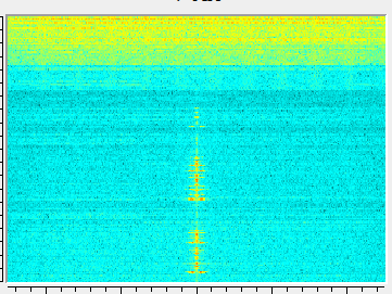

   

   Fig. 76 In the beginning the whole spectrum is hot, so we receive energy from the whole spectrum. Then rx_gain is gradually lowered. The spectrum becomes colder and we hear less noise. However, the signal is still not visible. When we increase tx_gain, then we can observe the contrast between cold and hot and the signal is clearly audible.

2. You hear the signal twice.

   We can reduce rx_gain to reduce the interference. Alternatively, we can increase the distance between the devices.

3. The signal is louder with a longer antenna.

Telecommunication

Solution to Exercise 17

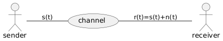
Typically no. Additionally, we have noise:

Solution to Exercise 18

2 and 3.

1. no, because the original signal is not modified, but certain frequencies are blocked in the ear

2. yes, because the sound interface actively modifies the signal by clipping

3. yes, remember when your noise is blocked. The voice tract modifies the waves created by your vocal cords

Solution to Exercise 19

Wireless

• 👍 convenient, no puzzles with entangled cables in your pocket

• 👎 have to remember charging

Solution to Exercise 20

The signals can propagate through multiple paths until they reach our smartphone, e.g., they are reflected through surfaces.

Even atmosphere bends electromagnetic waves, both radio and visual light. The refraction decreases with higher altitude but the bending effect is higher for lower frequency waves – radio in our case. So radio LOS is slightly broader.

Radio waves under 3 MHz can additionally be propagated through earth, e.g., AM radio.

Solution to Exercise 21

much more reliable than wireless

Solution to Exercise 22

• guided: wired

• unguided: wireless

Solution to Exercise 23

• wired: reliable and maybe cheap

• wireless: convenience of high mobility

  • unique selling point for telemedicine

Solution to Exercise 24

1. string that connects the cans

2. The vibrations are guided by the string

3. The vibrations caused by speech are modulated on the string.

Solution to Exercise 25

Conducting: We supply a voltage. If the voltage is high, then we have a 1, else 0. When we encode information using binary code, we get a series of zeroes and ones, which we can then use to switch on or off the voltage.

Optical: The same principle applies to light, e.g., when the light is off, then we have a 0.

Solution to Exercise 26

We can encode a symbol using multiple bits. For example, using four different voltage levels per symbol, or in other words, per time slot. This would correspond to \(log_2(4) = 2\) bits per symbol.

Symbol rate is typically lower than the bandwidth due to the possibility of encoding a symbol with multiple bits. The other way around – spreading a single bit into multiple time slots – typically does not occur.

Solution to Exercise 27

\(\frac{9600 bits/s}{5 bits} = 1920 Baud\)

Solution to Exercise 28

\(log_2(5) ~= 2.32 bits/symbol\)

\(1000 symbols/s \ldot 2.32 bits/symbol = 2320 bits/s\)

Solution to Exercise 29

Two symbols:

1. dit (dot)

2. dah (dash)

A dah is three times the duration of a dit.

Solution to Exercise 30

if we increase signal to noise ratio \(\frac{S}{N}\) then we increase the bit rate.

Solution to Exercise 31

The theorem gives the maximum bit rate on a given frequency. Based on the bit rate requirements, we can know the carrier frequency that we at least require.

Solution to Exercise 32

I see a CE logo on most of the electric/electronic devices I have on my desk.

It is there, because a device sold in the EU must be tested according to CE requirements.

Solution to Exercise 33

1. 56000/3100 = 18.1 bit/s/Hz

2. Alone it does not mean anything. This measure is more useful as a comparison with another communication channel.

Wireless telecommunication

Solution to Exercise 34

1. Wearable devices typically do not require a high bit rate. At the same time, there can be hundreds of them on a hospital floor. IR and low-range Bluetooth or ZigBee come into play. We don’t want a high range, because then the devices may interfere each other.

   The data received will be stored in a base station and forwarded per Wi-Fi or Ethernet to the intranet/internet.

2. Wi-Fi and broadband internet access, because high quality video communication requires ~20-50 Mbit. If the hospital is on a rural area, where no broadband exists, then the municipality must pay attention that the patients have access to cellular network or better WiMAX.

3. Let us assume, drones require operator control and real-time video for landing. We need low-latency communication. WiMAX and cellular networks are the options.

4. High-range Bluetooth can be used, because it is wireless and it supports up 100m.

Solution to Exercise 35

ZigBee does not need a dedicated central router. ZigBee supports decentralized topologies like mesh.

Solution to Exercise 36

offers up to ~10 Gbit/s which is similar to the Wi-Fi 6’s maximum bandwidth.

Fig. 77
CC BY-SA 3.0. By Inductiveload, NASA. Source: Wikimedia Commons

Visible light has a frequency in \(10^12Hz\) range. On the other hand, Wi-Fi 6 operates in the 6 GHz \(~=10^10Hz\). Therefore, the statement could indeed be true in the future.

Solution to Exercise 37

Typically, choosing a high frequency is a good idea, because

• higher spectrum is less used

• higher frequency means more bandwidth

However, we know from the former figures that higher frequencies are more significantly attenuated by rainfall. We could

• use many links with reduced frequency

• we may reduce frequency in case of rainfall and prioritize important data

• use an alternative wireless backup like satellite

Solution to Exercise 38

• in clothes

  • against stealing

  • for easy checkout at the payment terminal

• public transportation card

• to collect toll in highways

Solution to Exercise 39

• we could track items, e.g., medicine, equipment or babies

• data communication for sensors

  • a passive tag may not be sufficient to power the sensory circuit

Digital modulation

Solution to Exercise 78

Phase and frequency.

Solution to Exercise 82

We cannot.

FSK changes frequency, but an IQ plot can only visualize phase and amplitude changes.

Solution to Exercise 79

After sampling, we multiply the sampled values with the carrier signal.

Fig. 78 Data showing 10 symbols at 1V and 2V. Each symbol is sampled 10 times. Each symbol uses three cycles of a sinusoid.

Source M. Lichtman | License: CC BY-NC-SA 4.0

Solution to Exercise 80

Yes, but not a practical one. We want to keep the distances equal for best noise protection.

Solution to Exercise 81

• 2-ASK: The left of the two constellations in the bottom

• 4-ASK: The right one, but the left-most symbol must be in the origin.

Fig. 79 Five ASK schemes.

Source M. Lichtman | License: CC BY-NC-SA 4.0

Frequency domain

Solution to Exercise 42

infinite

Time-frequency pairs

Solution to Exercise 43

A single cosine term with \(a=2, b=0, c=0\).

Time-frequency properties

Solution to Exercise 44

Scaling in time property: when we compress a signal in time (which increases its data rate), its frequency spectrum expands proportionally. Mathematically, if \(x(t) \leftrightarrow X(f)\) is a Fourier transform pair, then \(x(at) \leftrightarrow \frac{1}{|a|}X(\frac{f}{a})\) where \(a\) is the scaling factor.

Solution to Exercise 45

Convolution in time: multiplication in the frequency domain is equivalent to convolution in the time domain. Using this property we can simply filter signals by multiplicating the Fourier-transformed signal with a filter’s frequency response.

Fast Fourier transform (FFT)

Solution to Exercise 46

1. In digital signal processing, we work with discrete signals. FFT is an implementation of discrete Fourier transformation and we need it to do calculations in the frequency domain.

2. FFT is computationally more efficient.

Negative frequencies

Solution to Exercise 48

We cannot know. This depends on the frequency that our device is tuned to.

Order in time does not matter

Solution to Exercise 49

We have to sample in chunks instead of the whole length of the signal.

FFT in Python

Solution to Exercise 50

1. Its magnitude and phase.

2. abs(), cmath.phase() or in numpy np.abs(), np.angle()

Solution to Exercise 51

1. The output of FFT ranges from frequency \(0\) to \(N-1\), where positive frequencies come first and negative ones last. fftshift() is basically a circular shift (to the right or left). It orders our sequence so that the DC frequency 0 is in the middle and negative frequencies come first in the sequence.

2. This way the x axis values are in order. That is how we are used to visualize things.

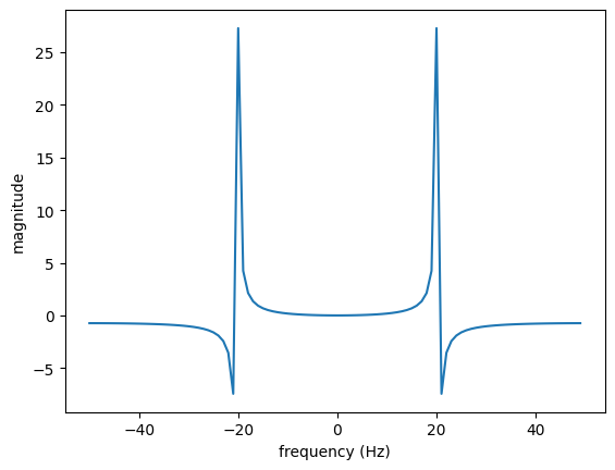
Solution to Exercise 52

-0.15 and 0.15.

This is a signal that has a period of 0.15, so we expect a peak at t=0.15 in the frequency domain. We have a real signal, which leads additionally to a peak at t=-0.15.

Plot:

import matplotlib.pyplot as plt
import numpy as np
from ipywidgets import interact
from numpy.fft import fft, fftshift, fftfreq

samp_freq = 100
timestep = 1  # in seconds
t = np.linspace(0, timestep, samp_freq)
y = np.sin(20 * 2 * np.pi * t)
Y = fftshift(fft(y))
freqs = fftshift(fftfreq(t.size, timestep/samp_freq))

plt.plot(freqs, Y)
plt.xlabel("frequency (Hz)")
plt.ylabel("magnitude")
plt.show()

Windowing

Solution to Exercise 53

If we multiply the original signal with a windowing function, the product will look similar to the shape of the windowing function. So the transformed windowing functions should also look similar to the transformed product signal.

In the frequency domain, we should compare the transformed blue rectangular window function to the others.

1. The rectangular window produces side lobes with higher magnitude while others less.

2. The left-most lobe has a greater width.

FFT sizing

Solution to Exercise 54

In sequence:

1. We cut the signal into smaller pieces

2. apply FFT on all pieces

3. we average them

Moreover, we don’t have to process every sample – we can skip a period before we FFT again.

Spectogram / waterfall

Solution to Exercise 55

My thoughts:

In a waterfall diagram, time is represented on the vertical axis. Each new FFT result is plotted at the top of the diagram (e.g., \(y=0\)), and older rows shift downward. This creates a visual effect resembling water flowing downwards.

Moreover, changes in the spectrum over time enhance the dynamic, flowing appearance, making the movement more pronounced.

I wanted to check my thoughts. I discovered here

The length of each vertical bar hanging below the horizontal axis increases as the plot moves to the right side of the graph, thus resembling a waterfall and giving the graph its name.

But this applies to 2D waterfall plots or charts. The simple 3D waterfall plot has mountain like shapes rather than a waterfall shape.

I did not research further. In the end I don’t know whether the inventor had similar ideas like mine.

Solution to Exercise 56

0.2 * np.random.randn(len(t))

Solution to Exercise 57

This is for decibel calculation. The signal is based on amplitude. To get a value proportional to the energy level, we have to square the signal.

FFT implementation

Solution to Exercise 58

Compare the indexes of \(x\) with the indexes of \(y\) on the right. We see on the right that the \(y\) with even indexes are on the top of the \(y\) with odd indexes.

IQ sampling

Sampling basics

Solution to Exercise 59

ADC

Solution to Exercise 60

\(S(nT)\), where \(n\) is an integer

Nyquist sampling

Solution to Exercise 61

We get constant values

Solution to Exercise 62

1. Twice the highest frequency that is available in the source signal.

2. Nyquist rate

Quadrature sampling

Solution to Exercise 63

A sinusoid with an angle and amplitude different than others

Complex numbers

Solution to Exercise 64

• \(A = 2\)

• \(\phi = -150 \deg = -\frac{5}{6} \pi\)

Solution to Exercise 65

It represents the phase of the signal

Complex numbers in FFTs

Solution to Exercise 66

1. Each complex number is associated with a cosine at a specific frequency. The real and complex components represent the amplitude and the phase of one cosine signal.

2. When we add these signals from 1., we hopefully get our original signal.

Receiver side

Solution to Exercise 67

Each sample corresponds to an \(I\) and a \(Q\) value. We have one million samples, so we get one million complex numbers and two million real numbers to work with.

Carrier and downconversion

Solution to Exercise 68

They correspond to the amplitude and phase of the received and downconverted signal. The sampled frequency bandwidth will be around the frequency \(f\).

Solution to Exercise 69

1. 10 GHz

2. Downconversion before sampling

Solution to Exercise 70

We tune the SDR to the carrier frequency.

Solution to Exercise 71

1. \(f = \frac{c}{\lambda}\), where \(c\) is the speed of light

2. \(\frac{\lambda}{2}\) or \(\frac{\lambda}{4}\)

Solution to Exercise 72

It elevates low-voltage signals to a readable level.

Baseband and bandpass signals

Solution to Exercise 73

A bandpass signal typically has frequencies around 0 Hz meaning both positive and negative frequencies. We cannot directly transmit negative or imaginary frequencies.

Solution to Exercise 74

The negative frequency is relative to the carrier frequency and its frequency becomes positive again after modulation. In other words, negative is relative to the carrier frequency.

Solution to Exercise 75

We can work at lower frequencies.

Digital modulation

Solution to Exercise 76

If we increase the frequency, then we need more bandwidth. The goal of modulation is to increase the data rate in a limited bandwidth.

Solution to Exercise 83

We will prove the equality of BER vs \(E_\mathrm{b}/N_0\) by proving that both the BER and \(E_\mathrm{b}/N_0\) the same for BPSK and QPSK.

BER:

• QPSK can be seen as two orthogonal BPSK signals (I and Q are orthogonal) transmitted simultaneously. Noise applies independently to both I and Q. So the bit error rate stays the same.

\(E_\mathrm{b}/N_0\):

• QPSK has double the spectral efficiency of BPSK, because QPSK has two bits per symbol, where BPSK only one bit. So QPSK has the twice the data rate in the same bandwidth and also uses twice the energy of BPSK per symbol. However \(E_\mathrm{b}\) looks at the energy per bit, which stays the same for both BPSK and QPSK.

Symbols

Solution to Exercise 77

1. 2 bit per 8 ns => 125 MHz * 2 bit = 250 Mbit/s

2. 4 16 symbols

3. \(\log_2 16\) 4 bits

4. 500 Mbit/s

Noise and dB

Gaussian noise

Solution to Exercise 85

We can model noise for simulation purposes.

Solution to Exercise 86

Mean of 2 and variance of 4 means that ~68% of the values will lie in the interval \([2-\sqrt{4}, 2+\sqrt{4}]\), but most of the numbers will be close to 2.

An example:

from numpy import array, random
signal = array([-5, -4, -3, -2, -1,  0,  1,  2,  3,  4])
noise  = array([+2, +3, +1, +0, +4, +1, -1, +2, +3, +5])
print("signal + noise:")
display(signal + noise)

# For comparing with actual random numbers
rng = random.default_rng()
noise_generated = rng.normal(loc=2, scale=2, size=10)  # loc: mean, scale: standard deviation

print("signal + noise_generated:")
signal + noise_generated

signal + noise:

array([-3, -1, -2, -2,  3,  1,  0,  4,  6,  9])

signal + noise_generated:

array([ 0.54740506, -2.44605084,  0.55729054,  0.73977707,  2.61110553,
        1.02712883,  2.17188941,  4.85967443,  3.91802359,  7.42582778])

Energy & power & duty cycle

Solution to Exercise 87

P_PROCESSOR = 5e-3  # W
P_TRANSCEIVER = 1e-3  # W
P_SLEEP = 1e-6  # W
DUTY_CYCLE = 5 / 100
AAA_CAPACITY = 900e-3  # Ah
AAA_VOLTAGE = 1.2  # V
aaa_energy = AAA_CAPACITY * 60 * 60 * AAA_VOLTAGE  # Ws
from sympy import symbols

p_p, p_t, p_s, d, e = symbols("P_p P_t P_s D E")
average_power = (p_p + p_t) * d + p_s * (1 - d)
print("average power:")
display(average_power)
print()

lifetime = e / average_power
print("lifetime:")
display(lifetime)
print()

lifetime_evald = lifetime.evalf(
    subs={
        p_p: P_PROCESSOR,
        p_t: P_TRANSCEIVER,
        p_s: P_SLEEP,
        d: DUTY_CYCLE,
        e: aaa_energy,
    }
)
print("evaluated:")
print(f"{int(lifetime_evald)} seconds")
print(f"{lifetime_evald/3600/24/30:.2f} months")

average power:

\[\displaystyle D \left(P_{p} + P_{t}\right) + P_{s} \left(1 - D\right)\]

lifetime:

\[\displaystyle \frac{E}{D \left(P_{p} + P_{t}\right) + P_{s} \left(1 - D\right)}\]

evaluated:
12919089 seconds
4.98 months

Decibel (dB)

Solution to Exercise 88

1. 0 dBm is 1 mW => -10 dBm = 0.1 mW => 0.0001 W

2. 0.5 W is half of 1 W

   for each doubling of halving we add or subtract ~3dB

   => 0.5 W = -3 dBW

3. 32 mW is 100 mW divided by roughly 4.

   => 100 mW = 0.1 W => 0.1 W = -10 dBW

   => 32 mW = -10 -3 -3 ~= -16 dBW

SNR

Solution to Exercise 89

1. -45 - (-90) = 45 dBm.

2. According to the dBm examples, a typical Wi-Fi signal has the power from -10 to -100 dBm. The value is in the middle and seems to be acceptable.

Link budget

Path loss

Solution to Exercise 90

Refer to this notebook.

Solution to Exercise 91

It is based on \(20 \log_{10}(c * \pi * 4)\).

For calculation, refer here: Free space path loss in decibels

Hata model

Solution to Exercise 92

Note that Hata model does not support 1800 MHz. We should use another model for this.

Refer to this notebook for the rest of the questions.

Indoor partition losses (same floor)

Solution to Exercise 93

Refer to this notebook.

Miscellaneous losses

Solution to Exercise 94

1. Typical distance in an urban area will be <1km. Mobile networks typically use 850–1900 MHz, so the loss will be less than 0.01 dB.

2. 0.01 dB is insignificant compared to the antenna gains

3. For example, satellite communications over many hundreds of km and 5G high-band >20 GHz.

ADS-B example

Solution to Exercise 95

We want at least 10 dB SNR. First let us calculate the minimum decodable receive power \(\min P_\mathrm{rx}\):

\[\begin{split}\min \mathrm{SNR} &= 10\,\mathrm{dB} \\ \min P_\mathrm{rx} &= 10\,\mathrm{dB} + (-140.8\,\mathrm{dBW}) = -130.8\,\mathrm{dBW}\end{split}\]

We want to get the maximum path loss \(\max L_\mathrm{path}\) from the minimum receive power \(\min P_\mathrm{rx}\):

\[\begin{split}\max L_\mathrm{path} &= \min P_\mathrm{rx} + 6\,\mathrm{dB} + 0\,\mathrm{dB} - 3\,\mathrm{dB} - 20\,\mathrm{dBW} \\ &= -147.8\,\mathrm{dB}\end{split}\]

Finally the maximum distance \(\max d\) using the FSPL formula:

\[\begin{split}\max d &= \max L_\mathrm{path} + 147.55\,\mathrm{dB} - 20 \log_{10} 1090e6\,\mathrm{dB} \\ &= \end{split}\]

from sympy import symbols
from math import log10
d, l_path = symbols('\\max{}d \\max{}l_\\mathrm{path}')
d = l_path + 147.55 - 20 * log10(1090e6)
display(d)
d_non_db = 10**(d/20)
L_PATH = 147.8
result_in_km = d_non_db.subs(l_path, L_PATH) /1000
print(f"~{int(result_in_km)} km")

\[\displaystyle \max{}l_\mathrm{path} - 33.1985299588125\]

~537 km

WBAN case studies

Solution to Exercise 97

• 50 % duty cycle => 15 mW

• assume 5 μW

• Values according to this this datasheet

  • typical means average daily conditions, nominal means test conditions.

  • assume nominal 35 mAh

  • 3.7V

LIR2032_ENERGY = 3.7 * 35 * 3600 * 10e-3
DUTY_CYCLE = 0.5
SLEEP_POWER = 5 * 10e-6
ACTIVE_POWER = 30 * 10e-3 * DUTY_CYCLE

def duration_in_h(duty_cycle=0.1):
    average_power = SLEEP_POWER * (1 - duty_cycle) + ACTIVE_POWER * duty_cycle
    return int(LIR2032_ENERGY / average_power / 3600)  # in h

for dc in (0.01, 0.1, 0.5):
    print(f"duty cycle: {dc} => {duration_in_h(dc)} days")

duty cycle: 0.01 => 835 days
duty cycle: 0.1 => 86 days
duty cycle: 0.5 => 17 days

We see that the sleep power plays a more significant role if the devices has to be operated for a long time.

Solution to Exercise 98

Humidity and blood pressure does not change rapidly, but acceleration can. So humidity must be sampled more frequently than accelerometer. Moreover accelerometer may need more precision (i.e., more decimal places) than humidity.

Solution to Exercise 99

• implants may not fail, i.e., they can be seen as mission-critical devices. Using the dedicated spectrum (medical implant communication service spectrum) avoids interference.

• S3 does not seem to have any special requirements

• S4 typically connects to a cellular or WLAN, which use frequencies >900 MHz.

Solution to Exercise 100

Wireless systems use avoidance (CA), because detection requires concurrent reception and transmission.

Solution to Exercise 101

0. Battery life and processing power limited, no external security threats exist. Communication takes place in a controlled environment (all wireless participants are known).

   E.g., a device tested in a research lab.

1. Battery life and processing power limited, identification of the participants is important, but data is not confidential.

   E.g., the patients have wearable access bands to get access to different rooms or to identify themselves using the id of the band (no person identifiable data involved).

2. Private data.

   E.g., biomarkers like heart-rate, ECG.

Solution to Exercise 102

1. The ASIC by Wang et al. has the lowest transmission power and have the highest data rate (maximum throughput). It has the highest \(\frac{\mathrm{data rate}}{power}\) ratio.

2. We see that this device has the lowest process technology in nanometers. Chips with less process technology numbers allow manufacturing of smaller transistor sizes and smaller transistors consume less energy.