
Link budget#
Learning goals
understand the significance of link budget and its components
calculate the link budget and minimum transmission power for a given scenario
evaluate the applicability of a path loss model to a given scenario
Introduction#
- link budget
Accounting of all of the power gains and losses that a communication signal experiences
describes one direction of the wireless link
link budget for transmission can be different than reception
result is SNR
Question: Is SNR high enough?
Signal power budget#
Given: transmit power
Wanted: received power

Fig. 60 A transmitter sends data. Receiver is waiting for data.#
Source M. Lichtman | License: CC BY-NC-SA 4.0
We need the following parameters to get the received power
\(P_\mathrm{tx}\) transmit power (dBW)
\(G_\mathrm{tx}\) gain of the transmitter antenna (dBi)
\(L_\mathrm{path}\) path loss (dB)
\(G_\mathrm{rx}\) gain of the receiver antenna (dBi)
\(L_\mathrm{misc}\) other miscellaneous losses like cables, connectors, atmospheric etc

Fig. 61 The parameters that determine the link budget are shown between a transmitter and receiver.#
Source M. Lichtman | License: CC BY-NC-SA 4.0
Transmit power \(P_\mathrm{tx}\)#
Measured in dB or dBm. Examples:
Power |
|
|---|---|
Bluetooth |
10 mW (-20 dBW) |
WiFi |
100 mW (-10 dBW) |
LTE base-station |
1 W (0 dBW) |
FM station |
10 kW (40 dBW) |
Antenna gains \(G_\mathrm{tx}\), \(G_\mathrm{rx}\)#
- gain (antenna)
a performance parameter that combines antenna’s directivity and radiation efficiency.
- directivity
parameter of an antenna or optical system which measures the degree to which the radiation emitted is concentrated in a single direction
- radiation efficiency
a measure of how well a radio antenna converts the radio-frequency power accepted at its terminals into radiated power and vice-versa.
In other words, how efficient is the antenna in terms of directing and converting the energy so that the communication can be successful.
Two main categories:
omnidirectional (no specific direction, in all directions)
directional
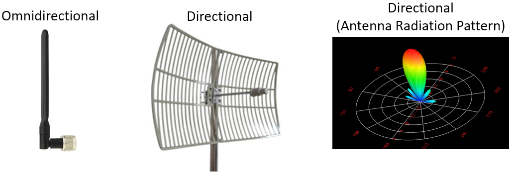
Fig. 62 Two antennas on the left and the radiation pattern of the directional antenna on the right.#
Source M. Lichtman | License: CC BY-NC-SA 4.0
Tip
Rule of thumb for antenna gains:
omnidirectional: 0-3 dB
directional: 5-60 dB
The directivity can be influenced both mechanically and electronically:
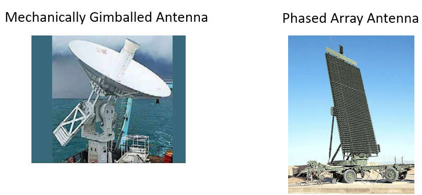
Fig. 63 The gimbal in the left picture maintains the same physical direction of the antenna even when the ship is swinging due to waves. The phased antenna on the right consists of many small antennas. Each of them is driven separately to achieve directivity.#
Source M. Lichtman | License: CC BY-NC-SA 4.0
Fig. 64 Phased array working principle. Even the antennas (A) are looking in the same direction, the direction \(\theta\) can be steered by individually driving the phase \(\phi\) of each antenna using the computer \(C\).
CC0. By Chetvorno. Source: Wikimedia Commons#
Phased array can be used in small scale too, which could be interesting for body sensors
Phased arrays can help to increase the \(G_\mathrm{tx}\) in higher frequencies, e.g., in 5G
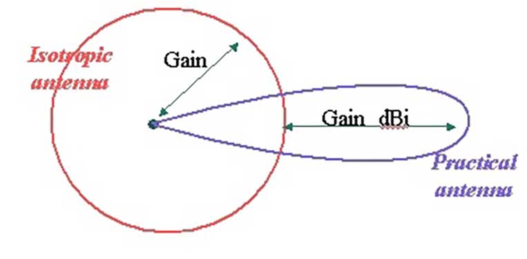
We assume that the antenna is pointing in the right direction for \(G_\mathrm{tx}\), \(G_\mathrm{rx}\)
it is measured in dBi, where i indicates that the gain is relative to an isotropic source
Path loss \(L_\mathrm{path}\)#
We had defined path loss here: path loss
given: a source emitting energy
wanted: how much energy goes through my receiving device?
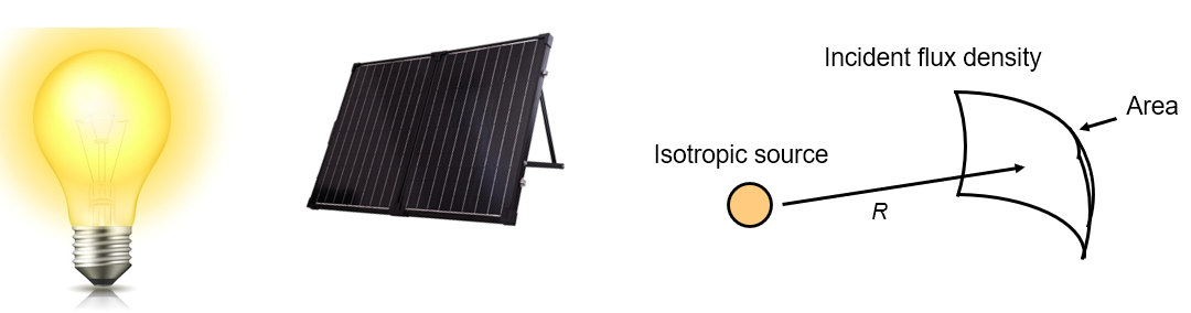
Fig. 65 On the left we see a light bulb and a solar panel. You may have observed on a solar-powered calculator that the energy produced by a solar panel will be less if the light source is more distant. The principle for this behavior is depicted on the right. The amount of rays going through a constant area will be less with increasing radius \(R\).#
Source M. Lichtman | License: CC BY-NC-SA 4.0
- flux
describes any effect that appears to pass or travel (whether it actually moves or not) through a surface or substance.
applies not only to electromagnetic waves but voice and light too.
There are different models for path loss. A simple one is the free-space path loss (FSPL).
Free-space path loss (FSPL)#
FSPL is based on Friis transmission equation.

Fig. 66 Portrayal of Harald T. Friis’ diagram from his article describing the physical components of the Friis Transmission Formula.
CC BY-SA 4.0. By John S. Huggins. Source: Wikimedia Commons#
He used the effective antenna areas in his original formula, but the contemporary version uses antenna gains instead. The ratio of received power \(P_r\) to the transmitted power \(P_t\) is:
\(\frac{P_r}{P_t} = D_t D_r \left(\frac{\lambda}{4\pi d}\right)^2\)
where:
\(D_t\) and \(D_t\) are the directivity of the transmitting and receiving antenna, respectively
a directivity of 1 means that a point source homogeneously distributes the energy in all directions, i.e., no directivity.
\(\lambda\) is the signal wavelength
\(d\) is the distance between the antennas
The inverse square term stems from the following geometry:

Fig. 67 A source emits a specific amount of rays, however the mount per unit area decreases exponentially with each linear distance increase \(r\)
CC BY-SA 3.0. By Borb (talk · contribs). Source: Wikimedia Commons#
An alternative figure for an isotropic radiator which visualizes the flow through a sphere.
The number of rays is distributed as follows: 4 units at a distance of \(2r\) and 9 units at a distance of \(3r\). Consequently, the signal density decreases exponentially with increasing distance.
The formula assumes that the antennas are in the far field of each other:

Fig. 68 The electromagnetic fields have different characteristics in the near and far field. Friis formula assumes far field.
Public domain. By Goran M Djuknic. Source: Wikimedia Commons#
If we focus on the free-space and leave the antenna effects out, we simplify Friis formula and get FSPL. This is why we probably have free-space in the acronym FSPL.
If we assume undirected antennas, then the directivities become 1. We want to calculate the loss, so we additionally flip the fraction and divide the power transmitted \(P_t\) by the power received \(P_r\).
\(\mathrm{FSPL} = (\frac{4\pi d}{\lambda})^2\)
The signal wavelength is the speed of light divided by the frequency. So we get:
\((\frac{4\pi d f}{c})^2\)
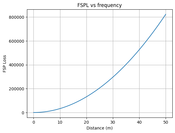
Let us try to understand its implications by analyzing the formula. We should observe that the loss grows exponentially in comparison to the linear growth of the distance and frequency. For example for 433 MHz:
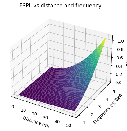
Let us analyze the loss for 433 MHz
If we convert FSPL to dB:
\(L_\mathrm{path,dB} = 20 \log_{10} d + 20 \log_{10} f - 147.55\)
Exercise 54
You are looking for a low-cost long range Wi-Fi antenna to connect two buildings. You focus on two options: CPE210 and CPE510. The buildings are about 20 km away from each other. Which one would you choose?
Browse the datasheet for these devices available on this page and look for relevant information.
Which information is relevant?
Which comparison metric could be most decisive?
Which one would you choose?
Hint
Calculating \(P_\mathrm{tx}\) could help.
Exercise 55
Where does the term -147.55 in the FSPL formula come from? Calculate.
Non-free-space models#
But we won’t have always free space or LoS. For indoors we have to use different modeling. Most frequencies go through walls, but not metal or thick brick or stone (masonry).
For a simple approximation we can stick to FSPL, however we should apply other models dependent on the environment.
Hata model#
path loss model in exterior environments
valid in range 150 - 1500 MHz
There are different formulas for urban environments of different sizes here.
Exercise 56
A telemedicine system transmits patient data wirelessly in the following scenario:
frequency 900 MHz
location Istanbul, the patient is moving in the city
patient antenna height 1.5 m
base station antenna height 50 m
What is the path loss for a 5 km link?
How does the loss change if the patient is 3 meter higher?
How does the loss change if the frequency is 1800 MHz?
Indoor partition losses (same floor)#
floors are typically partitioned (divided) by walls
Excerpt from Rappaport, 2024, Table 4.3:
Material type |
Loss (dB) |
Frequency |
Reference |
|---|---|---|---|
all metal |
26 |
815 MHz |
Cox83b |
Concrete wall |
8-15 |
1300 MHz |
Rap91c |
light textile |
3-5 |
1300 MHz |
Rap91c |
About glass partition and typical indoor losses from the company Ekahau
Typically, indoor glass partitions have somewhere between 1-3dB of attenuation and outdoor glass will have slightly more. Newer glass-heavy buildings, however, might have bomb-proof, RF shielded, or sound-proofed glass with attenuation as high as 16dB!
A typical interior wall that looks like drywall might have a nasty surprise inside that you don’t see. You knock on the wall, hear emptiness inside and assume 2-3dB attenuation. Then, you measure its true attenuation and reveal it is actually 12dB! Often, you will have a brick wall or sound-proofing material inside that ‘dry’ wall.
Exercise 57
Imagine you are analyzing the path loss at ~2 GHz in a modern building with:
glass partitions drawn as
---concrete walls drawn as
===.mobile devices 📱
base station 🛜
The following shows a single floor:
   <   5m   ><  5m   >< 5m    >
 ^ +--------+--------+--------+
 3m|   📱   |        |   📱   |
   |        |        |        |
 v +--------+        +--------+
   |   📱   |        |   📱   |
   |        |        |        |
   +========+========+========+
   |   📱   |   🛜   |   📱   |
   |        |        |        |
   +--------+        +--------+
   |   📱   |        |   📱   |
   |        |        |        |
   +--------+--------+--------+
What is the worst case path loss between the base station and a mobile device?
Optional: You want to simplify your calculations by finding the equivalent distances of partition walls. For example, you want to find the distance that corresponds to the attenuation of a concrete wall and add this equivalent distance to the path loss.
Does this idea make sense?
Hint
Partition losses are additional losses that are added to a free space loss.
Indoor partition losses between floors#
buildings are partitioned by floors
Average floor attenuation factors, excerpt from Seidel, 1992, Table II:
Building & Floors |
FAF (dB) |
σ(dB) |
|---|---|---|
Through 1 floor |
12.9 |
7.0 |
Through 2 floors |
18.7 |
2.8 |
Through 3 floors |
24.4 |
1.7 |
Through 4 floors |
27.0 |
1.5 |
ITU model for indoor attenuation#
useful for
a closed area inside a building delimited by walls.
Frequency: 900 MHz to 5.2 GHz
Floors: 1 to 3
\(L\): total path loss
\(f\): frequency
\(d\): distance
\(N\): distance power loss coefficient
\(n\): number of floors between the transmitter and receiver
\(P_\mathrm{f}(n)\): floor loss penetration factor
for the values \(N\) and \(P_\mathrm{f}(n)\), refer to the
Path loss models in ITU recommendation P.1238 : Propagation data and prediction methods for the planning of indoor radiocommunication systems and radio local area networks in the frequency range 300 MHz to 450 GHz. In version 2023 (12) you find it in section 3.
Log-distance path loss model#
inside a building or
densely populated areas over long distance
incorporates a random variable dependent on the fading

Fig. 69 Components of the signal attenuation in log-distance path loss model. In the diagram below, we see that the signal level will suffer from random fluctuations in addition to the deterministic path loss component. The fluctuations are caused by the objects in the environment which can cause constructive or destructive interference.
CC BY-SA 4.0. By Kirlf. Source: Wikimedia Commons#
Miscellaneous losses#
Includes:
cable, connector loss
antenna pointing imperfections
precipitation
atmospheric loss
Atmospheric loss is frequency dependent:

Fig. 70 Frequency dependent attenuation of electromagnetic radiation in atmosphere. Y axis shows attenuation in dB/km and x axis the frequency in GHz.
CC BY-SA 2.5. By No machine-readable author provided. Dantor assumed (based on copyright claims).. Source: Wikimedia Commons#
Exercise 58
How much is the attenuation for a typical mobile phone signal in an urban area? Use the attenuation-frequency diagram above.
Is this value significant compared to antenna gains?
Find a scenario which would suffer significantly from atmospheric loss.
Signal power equation#
Putting everything together:
\(P_\mathrm{rx} = P_\mathrm{tx} + G_\mathrm{tx} - L_\mathrm{path} + G_\mathrm{rx} - L_\mathrm{misc} \; \mathrm{dBW} \)
The calculation becomes a basic sum/subtraction. For example:
\(P_\mathrm{tx}\) = 1 W |
0 dBW |
\(G_\mathrm{tx}\) = 100 |
20 dB |
\(G_\mathrm{rx}\) = 1 |
0 dB |
\(L_\mathrm{path}\) |
-162.0 dB |
\(L_\mathrm{misc}\) |
-1.0 dB |
\(\Rightarrow P_\mathrm{rx}\) |
-143.0 dBW |
Effective radiated power (ERP)#
- Effective radiated power (ERP)
directional radio frequency power normalized to a half-wave dipole antenna
In other words: Amount of power a simple half-wave dipole antenna would need to transmit to produce the same signal strength as the actual antenna in its strongest direction.
Product of input power, antenna gain and miscellaneous losses like cable (\(P_\mathrm{tx} + G_\mathrm{tx} - L_\mathrm{cable}\) in dB).
- Effective isotropic radiated power
ERP but normalized to an isotropic source

Fig. 71 Two radiation patterns of an isotropic antenna \(R_\mathrm{iso}\)🟢 and a directed antenna \(R_\mathrm{a}\) ⚫, which illustrate the definition of EIRP. The flux emitted by the isotropic source is homogeneous in all directions as depicted by the green transparent sphere 🟢 \(R_\mathrm{iso}\). Both antennas are located in the origin. They have the same power flux density \(S\) in the direction of \(R_\mathrm{a}\)’s maximum signal strength. The transmitted power that must be applied to the isotropic antenna to achieve the same effect caused by \(R_\mathrm{a}\) is the EIRP.
CC0. By Chetvorno. Source: Wikimedia Commons#
Example: an FM radio station
if an FM radio station advertises 100 kW of power, this corresponds to the ERP and not the actual transmitter power.
\(P_\mathrm{tx}\) may be 10-20 kW \(\Rightarrow\) \(G_\mathrm{tx}\) 5-10 (7-10 dB).
EIRP may be more popular, but we can transform between them:
\(P_\mathrm{EIRP} = P_\mathrm{ERP} \cdot 1.64\) and \(P_\mathrm{EIRP} = P_\mathrm{ERP} + 2.15\) dB.
EIRP summarizes the transmit side of the link budget.
Thermal noise#
Using EIRP and path loss we got the \(P_\mathrm{rx}\), which is the received signal power. What about the noise? We need this for SNR.
Noise enters our communication link at the receiver. In other words, the signal is not corrupted, until we receive it. The noise does not reside in the air and disturb our signal, it comes from the fact that the signal amplifier on the receiver is not perfect and not at 0 Kelvin.
- thermal noise
noise generated by the thermal agitation of the charge carriers (usually electrons) inside an electrical conductor
Sensitive receivers like a radio telescope must be cooled down to decrease thermal noise.
A simple passive load at room temperature transfers a noise power of: (Rappaport, 2024, equation B.3)
\(k\) Boltzmann’s constant
\(T\) noise temperature, typically 290 K
not necessarily the room temperature
\(B\) signal bandwidth in Hz, assuming that the noise is filtered out
e.g., LTE signal that is 10 MHz wide \(\Rightarrow\) 10 MHz or 70 dBHz.
This gives the denominator (bottom term) of SNR.
SNR#
\(\mathrm{SNR} = \frac{P_\mathrm{rx}}{P_\mathrm{noise}}\)
\(\mathrm{SNR} = P_\mathrm{rx} - P_\mathrm{noise}\) (dB)
Typical goal: >10 dB.
We can get the SNR:
by looking at the FFT of the received signal.
calculating the power with and without the signal present.
The higher the SNR, the more signals you can receive (with insignificant amount of errors).
Link margin#
- link margin (LKM)
the difference between the minimum expected power received at the receiver’s end and the receiver’s sensitivity
- receiver’s sensitivity
the minimum power level at which the receiver can correctly decode the signal.
LKM represents the reliability and robustness of the link.
Example: Link budget of ADS-B#
- ADS-B
tech for determining an aircraft’s position
Used on flightradar24 by gathering signals from 40000 receivers around the world.
Stands for Automatic Dependent Surveillance–Broadcast
automatic: no pilot or external input required for transmission
dependent: but depends on data from the aircraft’s navigation system, in other words, it does not have a localization hardware itself.
Characteristics:
carrier: 1090 MHz
bandwidth: 2 MHz
modulation: PPM
data rate: 1 Mbit/s, one message every 56 - 112 µs
message size: 15 bytes
multiple messages are needed for the entire aircraft info
multiple access mechanism: messages are broadcast with a random period [0.4, 0.6] s
avoids collision of two or more airplanes messages
even two airplanes start transmitting at the same time, the second messages will likely not collide.
vertically polarized antennas
\(P_\mathrm{tx} \approx 100 \mathrm{W} = 20 \mathrm{dBW}\)
transmitter antenna: omnidirectional pointed downward
assume \(G_\mathrm{tx}\) about 3 dB
receiver antenna: omnidirectional
assume 0 dB
\(L_\mathrm{path}\) depends on the distance. Assuming 30 km between us and the airplane:
We won’t have free space
add 3 dB \(L_\mathrm{misc}\)
Assume that our antenna is well matched and there are no cable & connector issues.
However, we have interference from the base station nearby
add another 3 dB \(L_\mathrm{misc}\)
\(P_\mathrm{tx}\) |
20 dBW |
\(G_\mathrm{tx}\) |
3 dB |
\(G_\mathrm{rx}\) |
0 dB |
\(L_\mathrm{path}\) |
-122.7 dB |
\(L_\mathrm{misc}\) |
-6 dB |
\(P_\mathrm{rx}\) |
-105.7 dBW |
Thermal noise:
\(B\) = 2 MHz = 63 dBHz
\(T \approx\) 24.8 dBK, assuming 300K (27 degrees Celsius)
\(k =\) -228.6 dBW/K/Hz
Attention
In the SNR formula above we subtracted to dBW values and got dB in return. Even dBW is in relation to 1 W, SNR divides two dBW values to calculate their ratio. When we divide two dBW values, the unit W goes away and we get dB.
Our link margin in the classroom is roughly 35 dB. This is pretty huge, because ADS-B should work over much longer distances. You probably want to see another airplane much far away as a pilot.
In a classroom, the signal will still be weaker though, due to:
a poorly matched antenna
if the impedance of the transmission line is not equal to the RF source (typically 50 Ohm)
if we use the standard antenna provided by the kit, then the antenna should be already matched.
strong base stations or FM stations causing interference
These could lead 20-30 dB of extra losses.
Exercise 59
Assume we need at least 10 dB of SNR. What is the longest distance over that we can receive ADS-B signals?