
Frequency domain#
Intro#
SDR
as a concept: to perform signal processing of radio signals using software
as a device: hardware that receives or transmits data for SDR software
DSP
digital processing of signals
Frequency domain#
signals are in the time domain in their natural form
we cannot sample a signal in the freq. domain
interesting stuff happens in the frequency domain
Fourier series#
any signal can be represented by summing together sine waves.
Exercise 108
You want to approximate the following signals by summing up sine waves with different frequencies. Which one requires more sine waves than others?
a constant signal like \(f(x) = 1\)
a sawtooth
an irregular signal like this
Exercise 109
\(f(x) = a \cos (b \cdot x + c)\)
Match each variable to its corresponding concept in signal processing:
\(a\) represents the _________
\(b\) is related to the _________
\(c\) determines the _________
delay
amplitude
phase
frequency
Time-frequency pairs#
Exercise 110
How many sine signals do we need to model an impulse signal?
a quick change in the time domain result in many frequencies occurring
Exercise 111
How would you model a constant signal \(f(x) = 2\) using a sum of cosine waves (sum of many \(a \cos(b\cdot x + c)\))?
Fourier transform#
time domain \(x(t)\)
frequency domain \(X(f)\)
Time-frequency properties#
linearity
if we add two scaled signals in the time domain, then the addition and the scaling factors remain
frequency shift
if I multiply a signal with a complex exponential signal \(e^{2 \pi j f_0 t}\), then this corresponds to a positive shift in the frequency domain of \(f_0\).
frequency shift is very useful for modulation
scaling in time
if we compress the signal in the time domain using a factor of \(a\) (we increase the derivation), then the signal expands in the frequency domain. In other words, we increase the derivation and thus the frequency in the time domain and thus we need more and higher frequency components in the frequency domain
convolution in time
convolution creates a new signal
convolution in time corresponds to a multiplication in the frequency domain
convolution in frequency
we can reverse the operation
Exercise 112
The higher the data rate, the more spectrum bandwidth we require.
This fundamental relationship in signal processing is best explained by which time-frequency property of Fourier transforms?
linearity
frequency shift
scaling in time
convolution in time
Exercise 113
Which time-frequency property is most relevant when we want to mask or filter parts of a signal in the time domain?
linearity
frequency shift
scaling in time
convolution in time
imagine you want to get rid of a high frequency component of a signal.
=> define a windowing function in the frequency domain and transform it to the time domain.
Fast Fourier transform (FFT)#
FFT is an algorithm to compute the discrete Fourier transform
Exercise 114
What is the significance of the fast FT (FFT) in digital systems?
Why is it preferred over the standard discrete FT (DFT)?
if I put \(x\) samples into the FFT, I get \(x\) values out. What each component means is based on the sample rate.
when we use more samples, our resolution in the frequency domain increases
however, we don’t see more frequencies
we have to increase the sample rate for this
Exercise 115
If we put \(n\) samples into the FFT, we get \(n\) values out, which represent different frequencies available in the time domain.
You want to see higher frequency components of your input signal, e.g., not only see up to 100 MHz, but 200 MHz. What would you do?
A. Increase sampling frequency B. Decrease sampling frequency C. Increase the number of samples D. Decrease the number of samples
if the sampling rate is 1 MHz, then we will see signals up to 500 kHz.
each bin corresponds to \(f_s / N\) and in case of real signals, the diagram is symmetrical
Negative frequencies#
natural signals do not have a negative frequency
negative frequency is just a representation in the frequency domain
a negative frequency is a frequency lower than the center frequency
Exercise 116
Which absolute frequency range do we get with an SDR if we sample at a rate of 10 MHz?
Order in time does not matter#
Exercise 117
FFT does not care whether a specific frequency component came first or last.
How would you distinguish a signal and its mirrored version, which is flipped along the vertical axis using FFT?.
FFT in Python#
We will try to understand and visualize some aspects of FFT using Python.
Tip
If you don’t have a Python environment, you can use the web-based JupyterLite. It comes with numpy and matplotlib libraries pre-installed, which we will use.
Try the following code.
%pip install ipywidgets
import matplotlib.pyplot as plt
import numpy as np
from ipywidgets import interact
from numpy.fft import fft, fftshift


@interact
def plot(samp_freq=100):
    t = np.linspace(0, 1, samp_freq)
    y = np.sin(2 * np.pi * 5 * t) + np.sin(2 * np.pi * 10 * t)
    Y1 = fft(y)
    plt.plot(Y1, label="fft")

    Y2 = fftshift(fft(y))
    plt.plot(Y2, label="fftshift(fft)")

    plt.xlabel("frequency (Hz)")
    plt.ylabel("magnitude")
    plt.legend()
    plt.show()
np.fft.fft(s)Warning about the x values in
fftandfftshift(fft): FFT begins at frequency=0 continues up to N-1, however the frequencies N/2 up to N-1 represent negative frequencies from -N/2 to 0. Infftshiftedcase, the frequencies are arranged from -N/2 to -N/2-1.
Exercise 118
You want to visually make sense of a complex number. Which two properties of complex numbers are useful for this?
How can we get these properties in Python?
Exercise 119
What does the function
np.fft.fftshift()do?Why do we want to use this function?
Exercise 120
You apply fft() and fftshift on np.sin(20 * 2 * np.pi * t). At which t value/s do we get a peak/s?
Windowing#
FFT assumes that the sample we provide repeats itself. If the end of the signal does not match the beginning, then we get a sudden transition. This in turn introduces high-frequency components that are not actually present in the original signal.
solution: multiply with a function that has its high in the middle and smoothly decreases towards sides.
Exercise 121
We apply windowing to get rid frequencies that not actually present in our signal.
Where do you see the effect of windowing in the frequency plot on this figure
we can stick to the Hamming window
FFT sizing#
best FFT size is an order of 2
common sizes: 128 to 4096
Exercise 122
The common sizes for FFT are between 128 and 4096. Otherwise the FFT computation may take too long. Imagine you have much more than 4096 samples. How would you transform the signal using FFT?
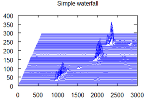
Spectogram / waterfall#
a visualization of spectrum
-
typically the spectrum shows 2D data – magnitude over frequency
bunch of FFT spectrums stacked together
if we want to visualize these 2D data over time, then our data has three dimensions
we could visualize the data using a heatmap
alternatively, we can use three axes like this. This is a waterfall plot.
not to be confused with waterfall charts. More info here
Exercise 123
Where could the word waterfall in waterfall plot come from?
Exercise 124
The following code creates a sequence of values that represent a signal with frequency f.
import numpy as np
import matplotlib.pyplot as plt

samp_rate = 1e6
t = np.arange(1024*1000) / samp_rate
f = 50e3 # Frequency of the tone
x = np.sin(2 * np.pi*f*t) + 0.2 * np.random.randn(len(t))
plt.plot(t[:200], x[:200])
plt.show()
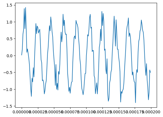
Which component represents the noise?
Exercise 125
The following is an excerpt from a spectrogram code:
spectrogram[i,:] = 10*np.log10(...**2)
Why do we square the signal?
FFT implementation#
Optional:
Exercise 126
Compare this representation with the FFT implementation below:
import numpy as np

def fft(x):
    N = len(x)
    if N == 1:
        return x
    twiddle_factors = np.exp(-2j * np.pi * np.arange(N//2) / N)
    x_even = fft(x[::2])
    x_odd = fft(x[1::2])
    return np.concatenate([x_even + twiddle_factors * x_odd,
                           x_even - twiddle_factors * x_odd])
The implementation breaks the input into x_even and x_odd and applies FFT separately on these components. If a scalar is reached, then it applies the butterfly operations and returns an array (by concatenation).
Where in the diagram do we see that the results of the inputs with even indexes are concatenated with results of inputs with odd indexes?